Intro to Raster Data
Last updated on 2024-03-12 | Edit this page
WARNING
Warning in
download.file("https://www.naturalearthdata.com/http//www.naturalearthdata.com/download/110m/physical/ne_110m_graticules_all.zip",
: cannot open URL
'https://www.naturalearthdata.com/http//www.naturalearthdata.com/download/110m/physical/ne_110m_graticules_all.zip':
HTTP status was '500 Internal Server Error'
ERROR
Error in download.file("https://www.naturalearthdata.com/http//www.naturalearthdata.com/download/110m/physical/ne_110m_graticules_all.zip", : cannot open URL 'https://www.naturalearthdata.com/http//www.naturalearthdata.com/download/110m/physical/ne_110m_graticules_all.zip'Overview
Questions
- What is a raster dataset?
- How do I work with and plot raster data in R?
Objectives
- Describe the fundamental attributes of a raster dataset.
- Explore raster attributes and metadata using R.
- Import rasters into R using the
terrapackage. - Plot a raster file in R using the
ggplot2package.
Things You’ll Need To Complete This Episode
See the lesson homepage for detailed information about the software, data, and other prerequisites you will need to work through the examples in this episode.
In this episode, we will introduce the fundamental principles, packages and metadata/raster attributes that are needed to work with raster data in R. We will discuss some of the core metadata elements that we need to understand to work with rasters in R, including CRS and resolution. We will also explore missing and bad data values as stored in a raster and how R handles these elements.
We will continue to work with the dplyr and
ggplot2 packages that were introduced in the Introduction to
R lesson. We will use two additional packages in this episode to
work with raster data - the terra and sf
packages. Make sure that you have these packages loaded.
R
library(terra)
library(ggplot2)
library(dplyr)
Introduce the Data
If not already discussed, introduce the datasets that will be used in this lesson. A brief introduction to the datasets can be found on the Geospatial workshop homepage.
For more detailed information about the datasets, check out the Geospatial workshop data page.
Open a Raster in R
Now that we’ve previewed the metadata for our GeoTIFF, let’s import
this raster dataset into R and explore its metadata more closely. We can
use the rast() function to open a raster in R.
First we will load our raster file into R and view the data structure.
R
DSM_HARV <-
  rast("data/NEON-DS-Airborne-Remote-Sensing/HARV/DSM/HARV_dsmCrop.tif")

DSM_HARV
OUTPUT
class       : SpatRaster
dimensions  : 1367, 1697, 1  (nrow, ncol, nlyr)
resolution  : 1, 1  (x, y)
extent      : 731453, 733150, 4712471, 4713838  (xmin, xmax, ymin, ymax)
coord. ref. : WGS 84 / UTM zone 18N (EPSG:32618)
source      : HARV_dsmCrop.tif
name        : HARV_dsmCrop
min value   :       305.07
max value   :       416.07
The information above includes a report of min and max values, but no other data range statistics. Similar to other R data structures like vectors and data frame columns, descriptive statistics for raster data can be retrieved like
R
summary(DSM_HARV)
WARNING
Warning: [summary] used a sampleOUTPUT
  HARV_dsmCrop
 Min.   :305.6
 1st Qu.:345.6
 Median :359.6
 Mean   :359.8
 3rd Qu.:374.3
 Max.   :414.7
but note the warning - unless you force R to calculate these
statistics using every cell in the raster, it will take a random sample
of 100,000 cells and calculate from that instead. To force calculation
all the values, you can use the function values:
R
summary(values(DSM_HARV))
OUTPUT
  HARV_dsmCrop
 Min.   :305.1
 1st Qu.:345.6
 Median :359.7
 Mean   :359.9
 3rd Qu.:374.3
 Max.   :416.1
To visualise this data in R using ggplot2, we need to
convert it to a dataframe. We learned about dataframes in an
earlier lesson. The terra package has an built-in
function for conversion to a plotable dataframe.
R
DSM_HARV_df <- as.data.frame(DSM_HARV, xy = TRUE)
Now when we view the structure of our data, we will see a standard dataframe format.
R
str(DSM_HARV_df)
OUTPUT
'data.frame': 2319799 obs. of 3 variables:
$ x : num 731454 731454 731456 731456 731458 ...
$ y : num 4713838 4713838 4713838 4713838 4713838 ...
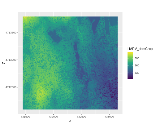
$ HARV_dsmCrop: num 409 408 407 407 409 ...We can use ggplot() to plot this data. We will set the
color scale to scale_fill_viridis_c which is a
color-blindness friendly color scale. We will also use the
coord_quickmap() function to use an approximate Mercator
projection for our plots. This approximation is suitable for small areas
that are not too close to the poles. Other coordinate systems are
available in ggplot2 if needed, you can learn about them at their help
page ?coord_map.
R
ggplot() +
    geom_raster(data = DSM_HARV_df , aes(x = x, y = y, fill = HARV_dsmCrop)) +
    scale_fill_viridis_c() +
    coord_quickmap()
Plotting Tip
More information about the Viridis palette used above at R Viridis package documentation.
See ?plot for more arguments to customize the plot
R
plot(DSM_HARV)
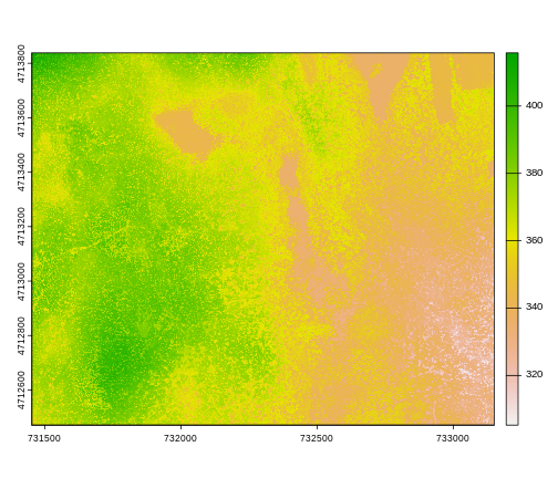
This map shows the elevation of our study site in Harvard Forest. From the legend, we can see that the maximum elevation is ~400, but we can’t tell whether this is 400 feet or 400 meters because the legend doesn’t show us the units. We can look at the metadata of our object to see what the units are. Much of the metadata that we’re interested in is part of the CRS. We introduced the concept of a CRS in an earlier lesson.
Now we will see how features of the CRS appear in our data file and what meanings they have.
Understanding CRS in Proj4 Format
The CRS for our data is given to us by R in proj4
format. Let’s break down the pieces of proj4 string. The
string contains all of the individual CRS elements that R or another GIS
might need. Each element is specified with a + sign,
similar to how a .csv file is delimited or broken up by a
,. After each + we see the CRS element being
defined. For example projection (proj=) and datum
(datum=).
UTM Proj4 String
A projection string (like the one of DSM_HARV) specifies
the UTM projection as follows:
+proj=utm +zone=18 +datum=WGS84 +units=m +no_defs +ellps=WGS84 +towgs84=0,0,0
- proj=utm: the projection is UTM, UTM has several zones.
- zone=18: the zone is 18
- datum=WGS84: the datum is WGS84 (the datum refers to the 0,0 reference for the coordinate system used in the projection)
- units=m: the units for the coordinates are in meters
- ellps=WGS84: the ellipsoid (how the earth’s roundness is calculated) for the data is WGS84
Note that the zone is unique to the UTM projection. Not all CRSs will have a zone. Image source: Chrismurf at English Wikipedia, via Wikimedia Commons (CC-BY).

Calculate Raster Min and Max Values
It is useful to know the minimum or maximum values of a raster dataset. In this case, given we are working with elevation data, these values represent the min/max elevation range at our site.
Raster statistics are often calculated and embedded in a GeoTIFF for us. We can view these values:
R
minmax(DSM_HARV)
OUTPUT
    HARV_dsmCrop
min       305.07
max       416.07
R
min(values(DSM_HARV))
OUTPUT
[1] 305.07R
max(values(DSM_HARV))
OUTPUT
[1] 416.07We can see that the elevation at our site ranges from 305.0700073m to 416.0699768m.