Sampling occurrence data with virtual data

Summary

• Description

• Getting ready

• Defining the Niche Space

• Virtual Data Generation

• Generating the Prediction Surface

• Sampling Virtual Data

  • Generating the Samples

  • Visualizing in E-Space

  • A Note on G-Space

---

Description

Virtual species are highly useful for controlled, purely theoretical experiments in quantitative ecology.

This vignette covers the workflow for simulating virtual species data entirely within environmental space (E-Space). This bypasses the need for geographic rasters, allowing you to generate and sample occurrence points directly from the mathematical properties of a defined niche ellipsoid.

Getting ready

First, we load the core packages required for our operations.

# Load packages
library(nicheR)
library(terra)

Defining the Niche Space

We define the fundamental niche based on our absolute environmental tolerances.

# Define environmental ranges (Min and Max)
range_df <- data.frame(bio_1  = c(22, 28),
                       bio_12 = c(1000, 3500),
                       bio_15 = c(50, 70))

# Build ellipsoid niche model
ell <- build_ellipsoid(range = range_df)
#> Starting: building ellipsoidal niche from ranges...
#> Step: computing covariance matrix...
#> Step: computing additional ellipsoidal niche metrics...
#> Done: created ellipsoidal niche.

Virtual Data Generation

virtual_data() Instead of applying our niche to a geographic map, we will simulate points drawn from the mathematical distribution of the niche itself.

Key Arguments

• object: A nicheR_ellipsoid object.

• n: The number of virtual points to generate within the environmental space.

• truncate: Logical. If TRUE, restricts the generated points to strictly fall within the ellipsoid’s confidence limits. If FALSE, points are drawn from a standard multivariate normal distribution.

• effect: Dictates the point distribution pattern.

  • "direct": Clusters points near the optimal centroid.

  • "inverse": Pushes points toward the marginal edges.

  • "uniform": Distributes points evenly throughout the volume (requires truncate = TRUE).

# Simulate 1,000 background virtual data points clustered near the center
virt_dat <- virtual_data(ell,
                         n = 1000,
                         truncate = FALSE,
                         effect = "direct",
                         seed = 1)

Generating the Prediction Surface

Now we score our simulated virtual data points to calculate their true habitat suitability and Mahalanobis distance. Notice that we pass our data frame (virt_dat) into the newdata argument instead of a raster.

# Predict suitability directly onto the virtual data frame
pred <- predict(ell,
                newdata = virt_dat,
                include_mahalanobis = TRUE,
                include_suitability = TRUE,
                suitability_truncated = TRUE,
                mahalanobis_truncated = TRUE,
                keep_data = TRUE) # Keeps the environmental variables attached
#> Starting: suitability prediction using newdata of class: matrix, array...
#> Step: Using 3 predictor variables: bio_1, bio_12, bio_15
#> Done: Prediction completed successfully. Returned columns: bio_1, bio_12, bio_15, Mahalanobis, suitability, Mahalanobis_trunc, suitability_trunc

Sampling Virtual Data

sample_virtual_data()

Objective: To sample virtual occurrence points from a non-spatial prediction data frame.

This function acts as the data-frame equivalent to sample_data(). It inherently supports the same weighting rules ("centroid", "edge", "random") and methods ("suitability", "mahalanobis").

Key Arguments

• virtual_prediction: The data frame output from the predict() function.

• prediction_layer: The name of the column containing the prediction metric to use as a sampling weight.

• sampling: Spatial bias of the sampling probability ("centroid", "edge", or "random").

• method: Weighting interpretation ("suitability" or "mahalanobis").

• strict: Logical. If TRUE, removes zero-valued rows before sampling. If NULL, auto-detects based on the column name or presence of zeros/NAs.

Generating the Samples

# Scenario 1: Suitability | Centroid | Strict = FALSE
occ_virt_suit_cent <- sample_virtual_data(n_occ = 100, 
                                          object = ell, 
                                          virtual_prediction = pred, prediction_layer = "suitability", 
                                          sampling = "centroid", 
                                          method = "suitability", 
                                          seed = 123)
#> Starting: sample_virtual_data()
#> Warning in resolve_prediction(virtual_prediction, prediction_layer):
#> 'prediction' is a data.frame, and it is missing 'x' and 'y', results wont show
#> geographical connections.
#> Done: sampled 100 points.

# Scenario 2: Suitability Truncated | Random | Strict = TRUE
occ_virt_suit_trunc_rand <- sample_virtual_data(n_occ = 100, 
                                                object = ell, 
                                                virtual_prediction = pred, 
                                                prediction_layer = "suitability_trunc", 
                                                sampling = "random",
                                                method = "suitability", 
                                                strict = TRUE, 
                                                seed = 123)
#> Starting: sample_virtual_data()
#> Warning in resolve_prediction(virtual_prediction, prediction_layer):
#> 'prediction' is a data.frame, and it is missing 'x' and 'y', results wont show
#> geographical connections.
#> Done: sampled 100 points.

# Scenario 3: Mahalanobis | Edge | Strict = FALSE
occ_virt_maha_edge <- sample_virtual_data(n_occ = 100, 
                                          object = ell, 
                                          virtual_prediction = pred, prediction_layer = "Mahalanobis", 
                                          sampling = "edge", 
                                          method = "mahalanobis",
                                          seed = 123)
#> Starting: sample_virtual_data()
#> Warning in resolve_prediction(virtual_prediction, prediction_layer):
#> 'prediction' is a data.frame, and it is missing 'x' and 'y', results wont show
#> geographical connections.
#> Done: sampled 100 points.

# Scenario 4: Mahalanobis Truncated | Centroid | Strict = TRUE
occ_virt_maha_trunc_cent <- sample_virtual_data(n_occ = 100, 
                                                object = ell, 
                                                virtual_prediction = pred, prediction_layer = "Mahalanobis_trunc", 
                                                sampling = "centroid",
                                                method = "mahalanobis", 
                                                strict = TRUE, 
                                                seed = 123)
#> Starting: sample_virtual_data()
#> Warning in resolve_prediction(virtual_prediction, prediction_layer):
#> 'prediction' is a data.frame, and it is missing 'x' and 'y', results wont show
#> geographical connections.
#> Done: sampled 100 points.

Visualizing in E-Space

Because our data points are already defined by their environmental values, we do not need to extract raster data. We can plot them directly into E-Space.

Dimension 1: Bio1 vs. Bio12

par(mfrow = c(2, 2), mar = c(4, 4, 3, 2)) 

# Plot 1: Suitability | Centroid | Strict = FALSE
plot_ellipsoid(ell, dim = c(1, 2), pch = ".", col_bg = "#9a9797", 
               xlab = "Bio1", ylab = "Bio12", main = "Virtual Suitability | Centroid | Strict = FALSE")
add_data(occ_virt_suit_cent, x = "bio_1", y = "bio_12", pts_col = "orange", pch = 20)
add_data(as.data.frame(t(ell$centroid)), x = "bio_1", y = "bio_12", pts_col = "red", pch = 15, cex = 1.5)

# Plot 2: Suit Truncated | Random | Strict = TRUE
plot_ellipsoid(ell, dim = c(1, 2), pch = ".", col_bg = "#9a9797", 
               xlab = "Bio1", ylab = "Bio12", main = "Virtual Suitability Trunc | Random | Strict = TRUE")
add_data(occ_virt_suit_trunc_rand, x = "bio_1", y = "bio_12", pts_col = "orange", pch = 20)
add_data(as.data.frame(t(ell$centroid)), x = "bio_1", y = "bio_12", pts_col = "red", pch = 15, cex = 1.5)

# Plot 3: Mahalanobis | Edge | Strict = FALSE
plot_ellipsoid(ell, dim = c(1, 2), pch = ".", col_bg = "#9a9797", 
               xlab = "Bio1", ylab = "Bio12", main = "Virtual Mahalanobis | Edge | Strict = FALSE")
add_data(occ_virt_maha_edge, x = "bio_1", y = "bio_12", pts_col = "orange", pch = 20)
add_data(as.data.frame(t(ell$centroid)), x = "bio_1", y = "bio_12", pts_col = "red", pch = 15, cex = 1.5)

# Plot 4: Mahalanobis Truncated | Centroid | Strict = TRUE
plot_ellipsoid(ell, dim = c(1, 2), pch = ".", col_bg = "#9a9797", 
               xlab = "Bio1", ylab = "Bio12", main = "Virt Mahalanobis Trunc | Centroid | Strict = TRUE")
add_data(occ_virt_maha_trunc_cent, x = "bio_1", y = "bio_12", pts_col = "orange", pch = 20)
add_data(as.data.frame(t(ell$centroid)), x = "bio_1", y = "bio_12", pts_col = "red", pch = 15, cex = 1.5)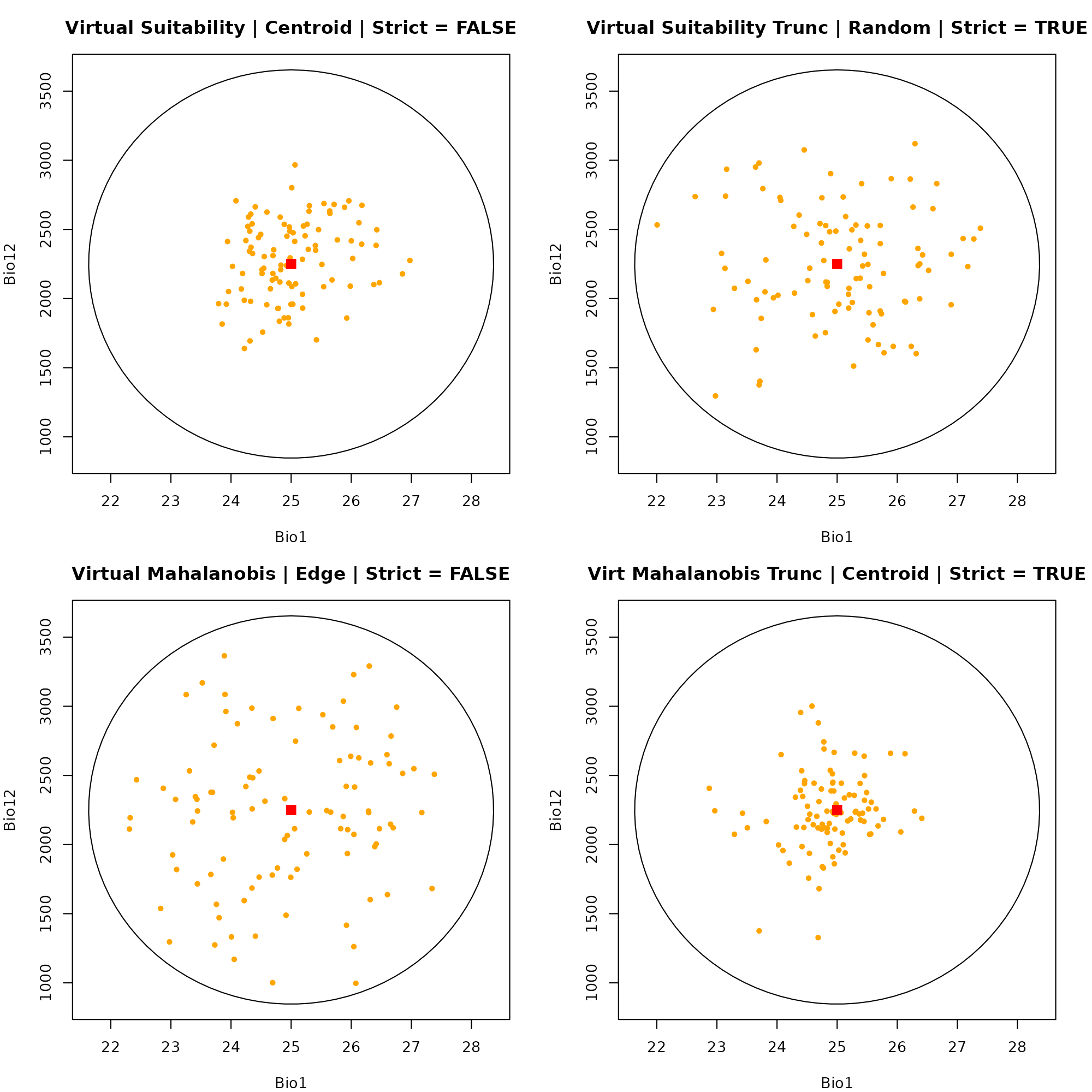

dev.off()
#> null device 
#>           1

Dimension 2: Bio1 vs. Bio15

par(mfrow = c(2, 2), mar = c(4, 4, 3, 2)) 
 
# Plot 1: Suitability | Centroid | Strict = FALSE
plot_ellipsoid(ell, dim = c(1, 3), pch = ".", col_bg = "#9a9797", 
               xlab = "Bio1", ylab = "Bio15", main = "Virtual Suitability | Centroid | Strict = FALSE")
add_data(occ_virt_suit_cent, x = "bio_1", y = "bio_15", pts_col = "orange", pch = 20)
add_data(as.data.frame(t(ell$centroid)), x = "bio_1", y = "bio_15", pts_col = "red", pch = 15, cex = 1.5)

# Plot 2: Suit Truncated | Random | Strict = TRUE
plot_ellipsoid(ell, dim = c(1, 3), pch = ".", col_bg = "#9a9797", 
               xlab = "Bio1", ylab = "Bio15", main = "Virtual Suitability Trunc | Random | Strict = TRUE")
add_data(occ_virt_suit_trunc_rand, x = "bio_1", y = "bio_15", pts_col = "orange", pch = 20)
add_data(as.data.frame(t(ell$centroid)), x = "bio_1", y = "bio_15", pts_col = "red", pch = 15, cex = 1.5)

# Plot 3: Mahalanobis | Edge
plot_ellipsoid(ell, dim = c(1, 3), pch = ".", col_bg = "#9a9797", 
               xlab = "Bio1", ylab = "Bio15", main = "Virtual Mahalanobis | Edge | Strict = FALSE")
add_data(occ_virt_maha_edge, x = "bio_1", y = "bio_15", pts_col = "orange", pch = 20)
add_data(as.data.frame(t(ell$centroid)), x = "bio_1", y = "bio_15", pts_col = "red", pch = 15, cex = 1.5)

# Plot 4: Mahalanobis Truncated | Centroid | Strict = TRUE
plot_ellipsoid(ell, dim = c(1, 3), pch = ".", col_bg = "#9a9797", 
               xlab = "Bio1", ylab = "Bio15", main = "Virt Mahalanobis Trunc | Centroid | Strict = TRUE")
add_data(occ_virt_maha_trunc_cent, x = "bio_1", y = "bio_15", pts_col = "orange", pch = 20)
add_data(as.data.frame(t(ell$centroid)), x = "bio_1", y = "bio_15", pts_col = "red", pch = 15, cex = 1.5)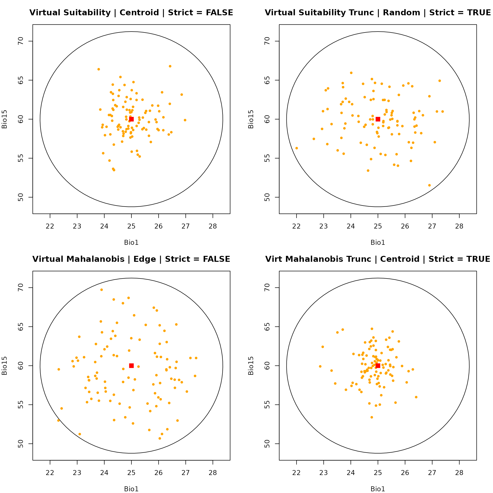

dev.off()
#> null device 
#>           1

A Note on G-Space

Because the virtual_data() function generates points purely based on statistical distributions within environmental dimensions (e.g., Temperature and Precipitation), these points do not possess spatial coordinates (Longitude/Latitude).

Consequently, pure virtual species simulated via this method exist exclusively in E-Space and cannot be directly plotted onto a geographic map (G-Space) without first projecting the niche model onto a physical landscape raster.