Generate occurrence data

Summary

Description
Getting ready
Part 1: Virtual Data
Part 2: Spatially-Explicit Occurrence Data
Part 3: Biased Occurrence Data
Save and export

Description

The nicheR package allows you to simulate how a species might be distributed by generating synthetic occurrence data from continuous prediction surfaces. This vignette progresses through three levels of complexity:

Virtual Data: Simulating species entirely within Environmental Space (E-Space), bypassing geographic rasters to test theoretical concepts.
Geographic Occurrence Data: Acting as a “virtual ecologist” to generate presence points across a physical landscape (G-Space) based on theoretical preferences.
Biased Occurrence Data: Introducing real-world collection bias (e.g., nighttime light, proximity to roads, species richness, land use land cover) to see how human sampling effort distorts our view of a species’ niche.

Getting ready

First, we load nicheR, this will also load terra as part of nicheR dependencies, alongside our pre-built fundamental niches and prediction layers. We will not be building models from scratch here; instead, we rely on data created in previous vignettes.

# Load packages
library(nicheR)

# Saving original plotting parameters
original_par <- par(no.readonly = TRUE)

# 1. Load environmental background raster
bios <- terra::rast(system.file("extdata", "ma_bios.tif", package = "nicheR"))

# 2. Load pre-calculated reference niches
data("ref_ellipse", package = "nicheR")  # 2D Niche (Bio1, Bio12)
data("example_sp_4", package = "nicheR") # 3D Niche (Bio1, Bio12, Bio15)

# 3. Load pre-calculated virtual backgrounds (E-Space only)
pred_virt_2d <- utils::read.csv(system.file("extdata", "predictions_virt.csv", package = "nicheR"))
pred_virt_3d <- utils::read.csv(system.file("extdata", "predictions_virt_3d.csv", package = "nicheR"))

# 4. Load pre-calculated geographic prediction surfaces
pred_2d <- terra::rast(system.file("extdata", "predictions_rast.tif", package = "nicheR"))
pred_3d <- terra::rast(system.file("extdata", "predictions_3d_rast.tif", package = "nicheR"))

# 5. Load pre-calculated biased prediction surfaces 
# (Habitat Suitability * Accessibility Bias)
bias_2d <- terra::rast(system.file("extdata", "applied_bias_rast.tif", package = "nicheR"))
bias_3d <- terra::rast(system.file("extdata", "applied_bias_3d_rast.tif", package = "nicheR"))

Part 1: Virtual Data

Virtual species are highly useful for controlled, purely theoretical experiments in quantitative ecology. Because the virtual_data() function generates points purely based on mathematical distributions, these points do not possess spatial coordinates (Longitude/Latitude). They exist exclusively in E-Space.

We will use the pre-calculated virtual backgrounds (pred_virt_2d and pred_virt_3d) loaded during our setup phase. These data frames contain 1,000 theoretical background points that have already been scored for suitability.

Basic generation

The virtual_data() function acts as the non-spatial twin to sample_data(). It picks “occurrences” from our virtual background.

occ_virt_basic <- virtual_data(object = ref_ellipse, n = 1000)

head(occ_virt_basic)
#>         bio_1   bio_12
#> [1,] 22.50672 1593.385
#> [2,] 22.20792 1795.909
#> [3,] 24.78859 1541.094
#> [4,] 22.63092 2148.820
#> [5,] 23.29214 1832.377
#> [6,] 25.65037 1544.886

Visualizing virtual data in 2D

Since virtual data lacks Geography, we visualize it exclusively in E-Space. The gray dots are our 1,000 background points. The orange dots are the 100 sampled individuals. Notice they cluster toward the center (red square) because higher suitability exists there.

plot_ellipsoid(ref_ellipse, dim = c(1, 2), pch = ".", col_bg = "#9a9797", 
               xlab = "Bio1 (Temp)", ylab = "Bio12 (Precip)", main = "Virtual E-Space")
add_data(occ_virt_basic, x = "bio_1", y = "bio_12", pts_col = "orange", pch = 20)
add_data(as.data.frame(t(ref_ellipse$centroid)), x = "bio_1", y = "bio_12", pts_col = "red", pch = 15, cex = 1.5)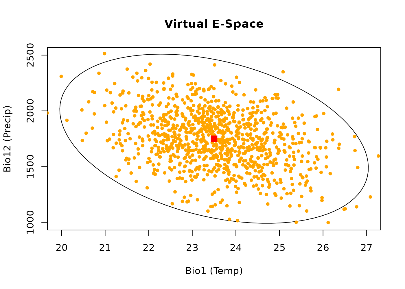

Three-dimensional virtual example

We can simulate pure virtual points across a 3-dimensional niche. The workflow is identical: generate a 3D background, score its suitability, and sample from it.

# Sample 100 virtual occurrences from the 3D background
occ_virt_3d <- virtual_data(
  n = 100, 
  object = example_sp_4
)

# Visualize across multiple dimensions in E-Space
par(mfrow = c(1, 2), mar = c(4, 4, 3, 2)) 

plot_ellipsoid(example_sp_4, dim = c(1, 2), pch = ".", col_bg = "#9a9797", main = "Virtual: Bio1 v Bio12")
add_data(occ_virt_3d, x = "bio_1", y = "bio_12", pts_col = "orange", pch = 20)
add_data(as.data.frame(t(example_sp_4$centroid)), x = "bio_1", y = "bio_12", pts_col = "red", pch = 15, cex = 1.5)

plot_ellipsoid(example_sp_4, dim = c(1, 3), pch = ".", col_bg = "#9a9797", main = "Virtual: Bio1 v Bio15")
add_data(occ_virt_3d, x = "bio_1", y = "bio_15", pts_col = "orange", pch = 20)
add_data(as.data.frame(t(example_sp_4$centroid)), x = "bio_1", y = "bio_15", pts_col = "red", pch = 15, cex = 1.5)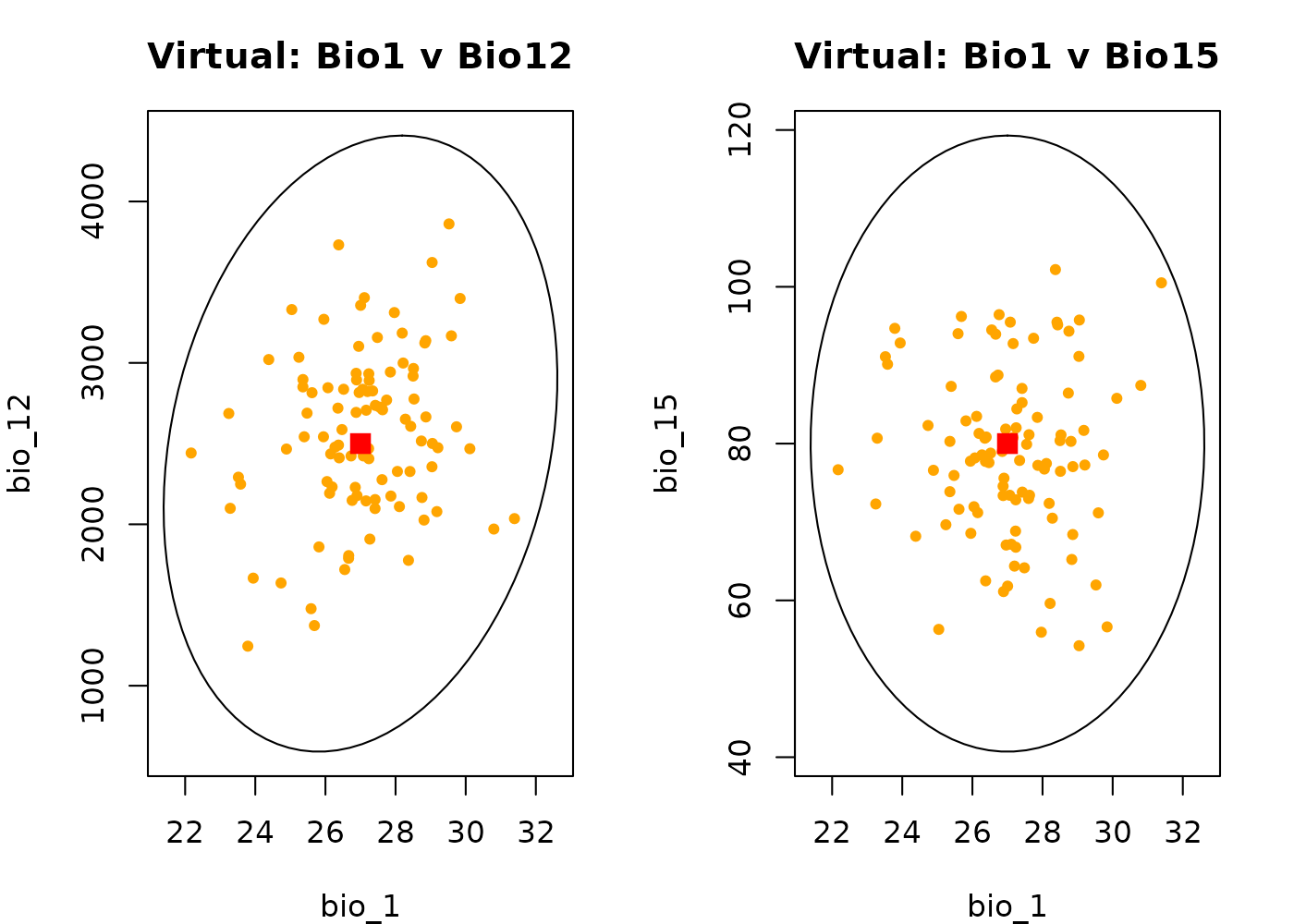

Part 2: Spatially-Explicit Occurrence Data

While virtual data exists solely in climate theory, sample_data() projects the niche onto a physical landscape raster. This generates spatial occurrences with physical coordinates (Longitude/Latitude) while simultaneously extracting their underlying environmental values. As a result, we can visualize and analyze these occurrences in both Geographic Space (G-Space) and Environmental Space (E-Space) at the same time.

Basic generation in 2D

Let’s generate 100 geographically grounded occurrences using the default suitability layer of our 2D prediction raster.

occ_geo_basic <- sample_data(
  n_occ = 100,
  prediction = pred_2d,
  prediction_layer = "suitability",
  seed = 123
)
#> Starting: sample_data()
#> Done: sampled 100 points.

par(mfrow = c(1, 2), mar = c(4, 4, 3, 2)) 

# 1. Geographic Space
terra::plot(pred_2d[["suitability"]], main = "G-Space: Geographic Map")
points(occ_geo_basic[, c("x", "y")], pch = 20, col = "red", cex = 1.2)

# 2. Environmental Space
plot_ellipsoid(ref_ellipse, background = as.data.frame(bios[[c("bio_1", "bio_12")]]), 
               dim = c(1, 2), pch = ".", col_bg = "#9a9797", main = "E-Space: Temp vs Precip")
add_data(occ_geo_basic, x = "bio_1", y = "bio_12", pts_col = "orange", pch = 20)
add_data(as.data.frame(t(ref_ellipse$centroid)), x = "bio_1", y = "bio_12", pts_col = "red", pch = 15, cex = 1.5)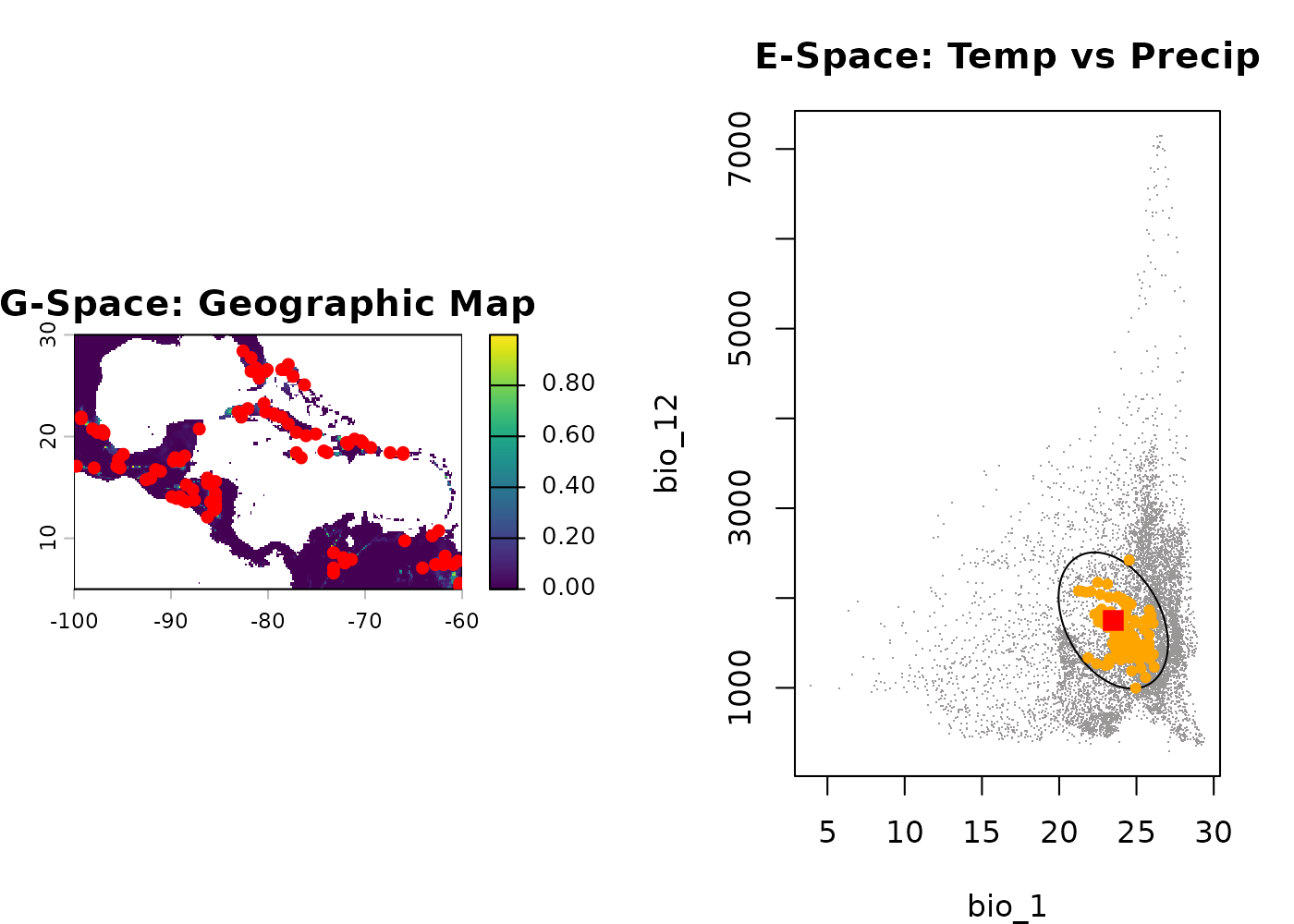

Effect of the `sampling` argument

The sampling argument determines the spatial bias of the selection probability.

centroid: Species strongly prefers optimal conditions (huddles near the center).
edge: Species is pushed into marginal environments (repelled to boundaries).
random: Uniform distribution across suitable habitats.

occ_cent <- sample_data(100, pred_2d, "suitability", sampling = "centroid", seed = 123)
#> Starting: sample_data()
#> Done: sampled 100 points.
occ_edge <- sample_data(100, pred_2d, "suitability", sampling = "edge", seed = 123)
#> Starting: sample_data()
#> 
#> Done: sampled 100 points.
occ_rand <- sample_data(100, pred_2d, "suitability", sampling = "random", seed = 123)
#> Starting: sample_data()
#> 
#> Done: sampled 100 points.

par(mfrow = c(3, 2), mar = c(3, 3, 2, 1), cex.main = 0.9) 

# Centroid
terra::plot(pred_2d[["suitability"]], main = "G-Space: Centroid Sampling"); points(occ_cent[, 1:2], pch = 20, col = "red")
plot_ellipsoid(ref_ellipse, background = as.data.frame(bios[[c("bio_1", "bio_12")]]), dim = c(1, 2), pch = ".", col_bg = "#9a9797", main = "E-Space: Centroid")
add_data(occ_cent, x = "bio_1", y = "bio_12", pts_col = "orange", pch = 20)

# Edge
terra::plot(pred_2d[["suitability"]], main = "G-Space: Edge Sampling"); points(occ_edge[, 1:2], pch = 20, col = "red")
plot_ellipsoid(ref_ellipse, background = as.data.frame(bios[[c("bio_1", "bio_12")]]), dim = c(1, 2), pch = ".", col_bg = "#9a9797", main = "E-Space: Edge")
add_data(occ_edge, x = "bio_1", y = "bio_12", pts_col = "orange", pch = 20)

# Random
terra::plot(pred_2d[["suitability"]], main = "G-Space: Random Sampling"); points(occ_rand[, 1:2], pch = 20, col = "red")
plot_ellipsoid(ref_ellipse, background = as.data.frame(bios[[c("bio_1", "bio_12")]]), dim = c(1, 2), pch = ".", col_bg = "#9a9797", main = "E-Space: Random")
add_data(occ_rand, x = "bio_1", y = "bio_12", pts_col = "orange", pch = 20)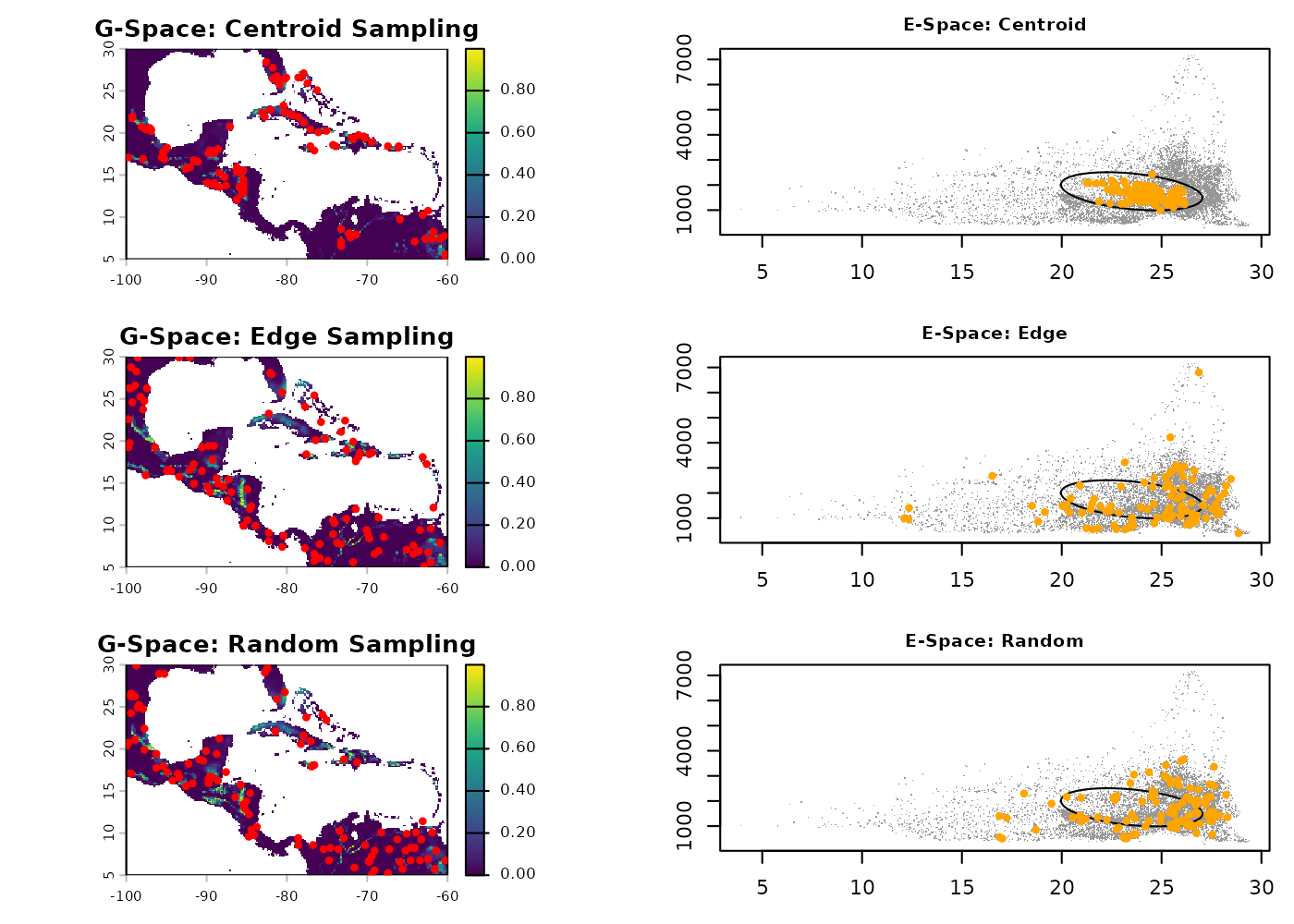

Effect of the `method` argument

The method argument controls the underlying mathematical weight used to draw the samples.

suitability: Weights linearly based on the 0-1 habitat suitability index.
mahalanobis: Weights based on the multivariate environmental distance, creating a stricter concentration in optimal environments.

occ_meth_suit <- sample_data(100, pred_2d, "suitability", method = "suitability", seed = 123)
#> Starting: sample_data()
#> Done: sampled 100 points.
occ_meth_maha <- sample_data(100, pred_2d, "Mahalanobis", method = "mahalanobis", seed = 123)
#> Starting: sample_data()
#> 
#> Done: sampled 100 points.

par(mfrow = c(2, 2), mar = c(3, 3, 2, 1), cex.main = 0.9) 

# Suitability
terra::plot(pred_2d[["suitability"]], main = "G-Space: Method = Suitability"); points(occ_meth_suit[, 1:2], pch = 20, col = "red")
plot_ellipsoid(ref_ellipse, background = as.data.frame(bios[[c("bio_1", "bio_12")]]), dim = c(1, 2), pch = ".", col_bg = "#9a9797", main = "E-Space: Suitability")
add_data(occ_meth_suit, x = "bio_1", y = "bio_12", pts_col = "orange", pch = 20)

# Mahalanobis
terra::plot(pred_2d[["Mahalanobis"]], main = "G-Space: Method = Mahalanobis"); points(occ_meth_maha[, 1:2], pch = 20, col = "red")
plot_ellipsoid(ref_ellipse, background = as.data.frame(bios[[c("bio_1", "bio_12")]]), dim = c(1, 2), pch = ".", col_bg = "#9a9797", main = "E-Space: Mahalanobis")
add_data(occ_meth_maha, x = "bio_1", y = "bio_12", pts_col = "orange", pch = 20)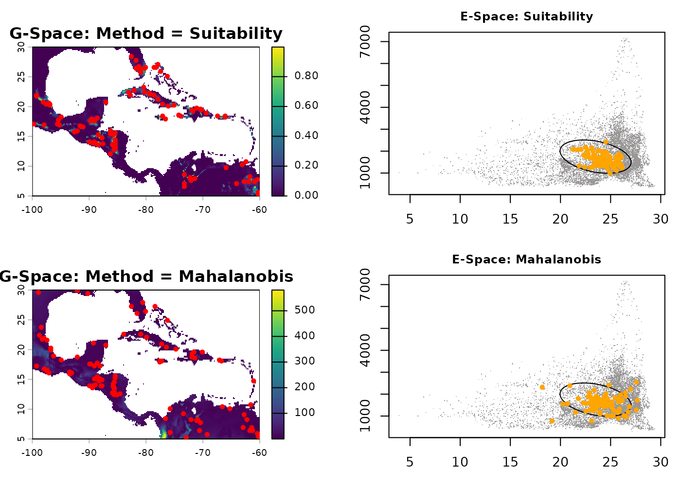

Effect of the `strict` argument

By default (strict = FALSE), generating occurrences allows points to fall slightly outside the strict boundaries of the fundamental niche to simulate sink populations. Setting strict = TRUE (using a truncated layer) establishes a hard boundary.

occ_lax <- sample_data(100, pred_2d, "suitability", strict = FALSE, seed = 123)
#> Starting: sample_data()
#> Done: sampled 100 points.
occ_strict <- sample_data(100, pred_2d, "suitability_trunc", strict = TRUE, seed = 123)
#> Starting: sample_data()
#> 
#> Done: sampled 100 points.

par(mfrow = c(2, 2), mar = c(3, 3, 2, 1), cex.main = 0.9) 

# Lax
terra::plot(pred_2d[["suitability"]], main = "G-Space: Strict = FALSE"); points(occ_lax[, 1:2], pch = 20, col = "red")
plot_ellipsoid(ref_ellipse, background = as.data.frame(bios[[c("bio_1", "bio_12")]]), dim = c(1, 2), pch = ".", col_bg = "#9a9797", main = "E-Space: Strict = FALSE")
add_data(occ_lax, x = "bio_1", y = "bio_12", pts_col = "orange", pch = 20)

# Strict
terra::plot(pred_2d[["suitability_trunc"]], main = "G-Space: Strict = TRUE"); points(occ_strict[, 1:2], pch = 20, col = "red")
plot_ellipsoid(ref_ellipse, background = as.data.frame(bios[[c("bio_1", "bio_12")]]), dim = c(1, 2), pch = ".", col_bg = "#9a9797", main = "E-Space: Strict = TRUE")
add_data(occ_strict, x = "bio_1", y = "bio_12", pts_col = "orange", pch = 20)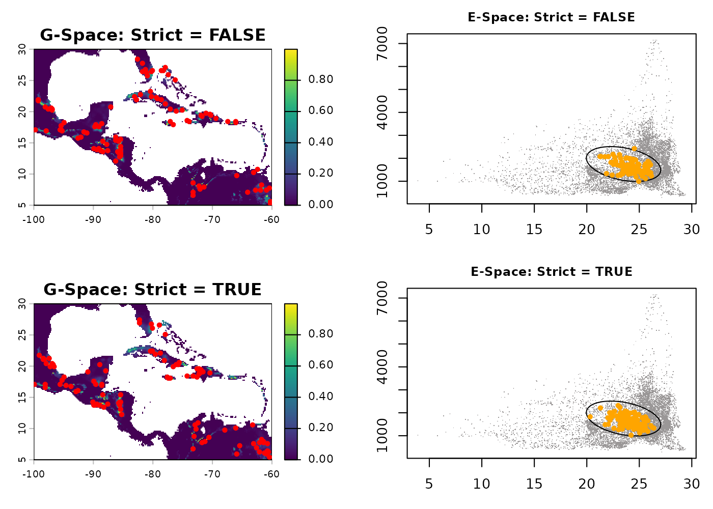

Three-Dimensional Example

Generating occurrences for a 3-dimensional niche operates exactly the same way. We simply pass the 3D prediction raster and view the outputs across multiple axes (e.g., Temperature vs. Precipitation, and Temperature vs. Seasonality).

occ_geo_3d <- sample_data(100, pred_3d, "suitability", seed = 123)
#> Starting: sample_data()
#> Done: sampled 100 points.

par(mfrow = c(1, 3), mar = c(4, 4, 3, 2)) 
terra::plot(pred_3d[["suitability"]], main = "G-Space: 3D Projection")
points(occ_geo_3d[, c("x", "y")], pch = 20, col = "red", cex = 1.2)

plot_ellipsoid(example_sp_4, background = as.data.frame(bios[[c("bio_1", "bio_12", "bio_15")]]), dim = c(1, 2), pch = ".", col_bg = "#9a9797", main = "E-Space: Bio1 v Bio12")
add_data(occ_geo_3d, x = "bio_1", y = "bio_12", pts_col = "orange", pch = 20)

plot_ellipsoid(example_sp_4, background = as.data.frame(bios[[c("bio_1", "bio_12", "bio_15")]]), dim = c(1, 3), pch = ".", col_bg = "#9a9797", main = "E-Space: Bio1 v Bio15")
add_data(occ_geo_3d, x = "bio_1", y = "bio_15", pts_col = "orange", pch = 20)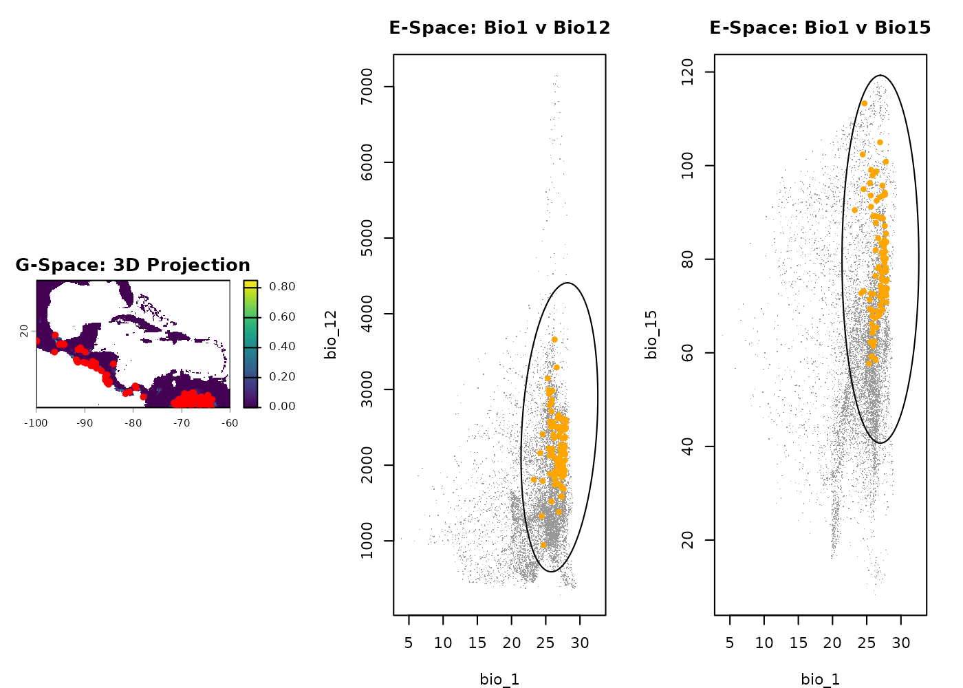

Part 3: Biased Occurrence Data

In the real world, species occurrence data is heavily influenced by human accessibility. If a model is trained on biased data, it will predict where the observers go, rather than where the species lives.

Using sample_biased_data(), we can draw points from a raster that has already been mathematically multiplied by a bias layer (e.g., nighttime light, distance to roads) to simulate this real-world distortion.

Basic biased generation in 2D

Once the spatial points are generated, we must use terra::extract() to pull the underlying climate values so we can plot them in E-Space and observe the distortion.

occ_bias_xy <- sample_biased_data(
  n_occ = 100, 
  prediction = bias_2d, 
  prediction_layer = "suitability_biased_direct", 
  strict = FALSE,
  seed = 123
)
#> Starting: sample_biased_data()
#> Done: sampled 100 points from biased prediction layer

# Extract environmental data at these coordinates to view E-space distortion
occ_bias_env <- terra::extract(bios, occ_bias_xy[, c("x", "y")])

par(mfrow = c(1, 2), mar = c(4, 4, 3, 2)) 
terra::plot(bias_2d[["suitability_biased_direct"]], main = "G-Space: Biased Map")
terra::points(occ_bias_xy[, c("x", "y")], pch = 20, col = "red", cex = 1.2)

plot_ellipsoid(ref_ellipse, background = as.data.frame(bios[[c("bio_1", "bio_12")]]), dim = c(1, 2), pch = ".", col_bg = "#9a9797", main = "E-Space: Distorted Niche")
add_data(occ_bias_env, x = "bio_1", y = "bio_12", pts_col = "orange", pch = 20)
add_data(as.data.frame(t(ref_ellipse$centroid)), x = "bio_1", y = "bio_12", pts_col = "red", pch = 15, cex = 1.5)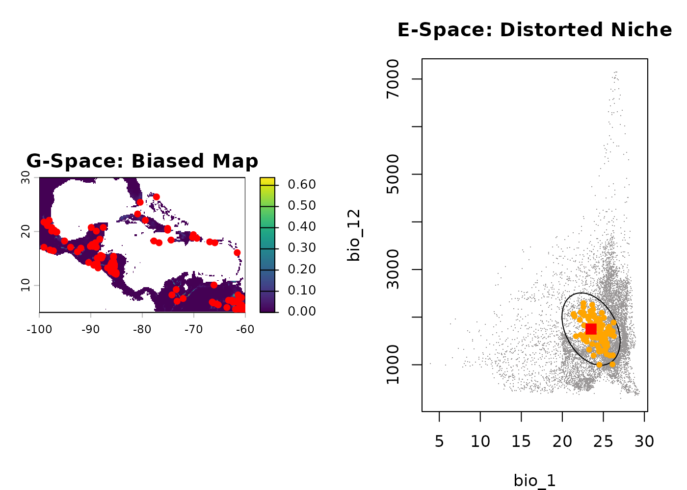

Notice the Distortion: Because observers only sampled accessible areas, the orange dots are dragged away from the optimal centroid (red square) and pushed into marginal climates.

Important Note: Why are there no sampling or method arguments? {#bias-no-sampling}

You might notice that sample_biased_data() is missing the sampling and method arguments found in sample_data().

This is mathematically intentional! In biased sampling, the prediction layer values themselves define exactly where points are drawn from. The raster acts as a direct, literal probability surface. Overlaying an artificial “edge” or “centroid” preference via an argument would undermine the spatial collection bias (e.g., roads) we are trying to simulate.

Effect of the biased `strict` argument

While we don’t control sampling strategies, we can control whether occurrences are allowed in zero-probability/NA cells. Setting strict = TRUE acts as a strict firewall, removing any NA and zero-valued pixels prior to pulling samples.

# strict = TRUE ensures sampling ONLY happens in explicitly positive bias areas
occ_bias_strict_xy <- sample_biased_data(100, bias_2d, "suitability_biased_direct", strict = TRUE, seed = 123)
#> Starting: sample_biased_data()
#> Done: sampled 100 points from biased prediction layer
occ_bias_strict_env <- terra::extract(bios, occ_bias_strict_xy[, c("x", "y")])

par(mfrow = c(1, 2), mar = c(4, 4, 3, 2)) 
terra::plot(bias_2d[["suitability_biased_direct"]], main = "G-Space: Biased Map (Strict)")
terra::points(occ_bias_strict_xy[, c("x", "y")], pch = 20, col = "red", cex = 1.2)

plot_ellipsoid(ref_ellipse, background = as.data.frame(bios[[c("bio_1", "bio_12")]]), dim = c(1, 2), pch = ".", col_bg = "#9a9797", main = "E-Space: Strict Bias")
add_data(occ_bias_strict_env, x = "bio_1", y = "bio_12", pts_col = "orange", pch = 20)

Three-Dimensional Biased Example

Finally, let’s look at biased sampling on a 3-dimensional niche (example_sp_4).

occ_bias_3d_xy <- sample_biased_data(100, bias_3d, "suitability_biased_direct", seed = 123)
#> Starting: sample_biased_data()
#> Done: sampled 100 points from biased prediction layer
occ_bias_3d_env <- terra::extract(bios, occ_bias_3d_xy[, c("x", "y")])

par(mfrow = c(1, 3), mar = c(4, 4, 3, 2)) 
terra::plot(bias_3d[["suitability_biased_direct"]], main = "G-Space: 3D Biased Map")
terra::points(occ_bias_3d_xy[, c("x", "y")], pch = 20, col = "red", cex = 1.2)

plot_ellipsoid(example_sp_4, background = as.data.frame(bios[[c("bio_1", "bio_12", "bio_15")]]), dim = c(1, 2), pch = ".", col_bg = "#9a9797", main = "E-Space: Bio1 v Bio12")
add_data(occ_bias_3d_env, x = "bio_1", y = "bio_12", pts_col = "orange", pch = 20)
add_data(as.data.frame(t(example_sp_4$centroid)), x = "bio_1", y = "bio_12", pts_col = "red", pch = 15, cex = 1.5)

plot_ellipsoid(example_sp_4, background = as.data.frame(bios[[c("bio_1", "bio_12", "bio_15")]]), dim = c(1, 3), pch = ".", col_bg = "#9a9797", main = "E-Space: Bio1 v Bio15")
add_data(occ_bias_3d_env, x = "bio_1", y = "bio_15", pts_col = "orange", pch = 20)
add_data(as.data.frame(t(example_sp_4$centroid)), x = "bio_1", y = "bio_15", pts_col = "red", pch = 15, cex = 1.5)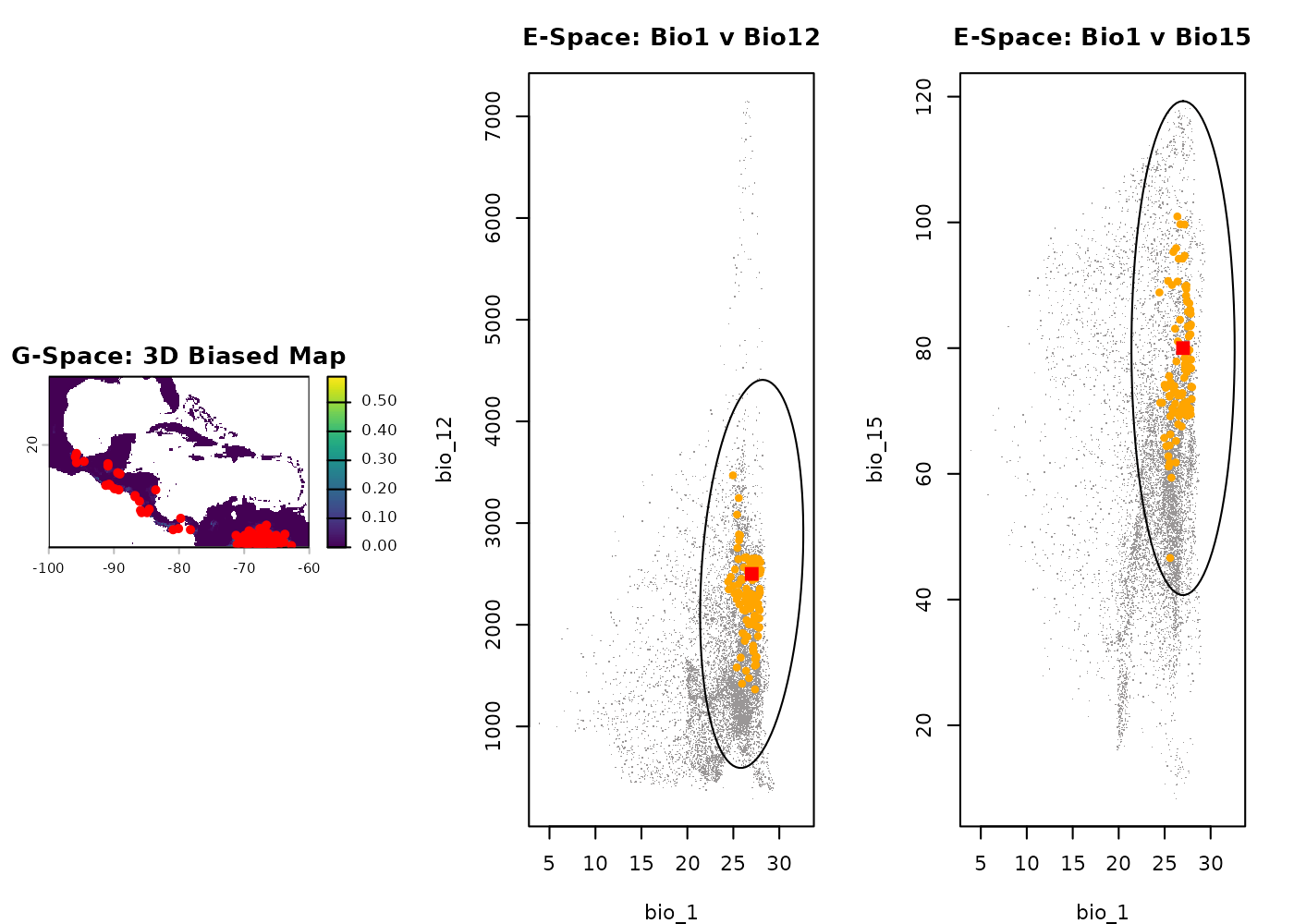

# Reset plotting parameters
par(original_par)

Save and export

Because we generated standard spatial coordinates and data frames, exporting these simulated datasets for testing model robustness or downstream analyses is straightforward.

# Save Pure Virtual Data
write.csv(occ_virt_basic, file = tempfile(), row.names = FALSE)

# Save Geographic Data
write.csv(occ_geo_basic, file = tempfile(), row.names = FALSE)

# Save Biased Data (combining XY and environmental data)
biased_final <- cbind(occ_bias_xy, occ_bias_env)
write.csv(biased_final, file = tempfile(), row.names = FALSE)